E-ask-how

Algorithm

PageRank is a probability distribution used to represent the likelihood that a person randomly clicking on links will arrive at any particular page. PageRank can be calculated for collections of documents of any size. It is assumed in several research papers that the distribution is evenly divided among all documents in the collection at the beginning of the computational process. The PageRank computations require several passes, called "iterations", through the collection to adjust approximate PageRank values to more closely reflect the theoretical true value.
A probability is expressed as a numeric value between 0 and 1. A 0.5 probability is commonly expressed as a "50% chance" of something happening. Hence, a PageRank of 0.5 means there is a 50% chance that a person clicking on a random link will be directed to the document with the 0.5 PageRank.

Simplified algorithm

Assume a small universe of four web pages: A, B, C and D. Links from a page to itself, or multiple outbound links from one single page to another single page, are ignored. PageRank is initialized to the same value for all pages. In the original form of PageRank, the sum of PageRank over all pages was the total number of pages on the web at that time, so each page in this example would have an initial PageRank of 1. However, later versions of PageRank, and the remainder of this section, assume a probability distribution between 0 and 1. Hence the initial value for each page is 0.25.
The PageRank transferred from a given page to the targets of its outbound links upon the next iteration is divided equally among all outbound links.
If the only links in the system were from pages B, C, and D to A, each link would transfer 0.25 PageRank to A upon the next iteration, for a total of 0.75.

$PR(A)= PR(B) + PR(C) + PR(D).\,$

Suppose instead that page B had a link to pages C and A, while page D had links to all three pages. Thus, upon the next iteration, page B would transfer half of its existing value, or 0.125, to page A and the other half, or 0.125, to page C. Since D had three outbound links, it would transfer one third of its existing value, or approximately 0.083, to A.

$PR(A)= \frac{PR(B)}{2}+ \frac{PR(C)}{1}+ \frac{PR(D)}{3}.\,$

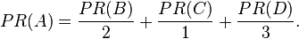
In other words, the PageRank conferred by an outbound link is equal to the document's own PageRank score divided by the number of outbound links L( ).

$PR(A)= \frac{PR(B)}{L(B)}+ \frac{PR(C)}{L(C)}+ \frac{PR(D)}{L(D)}. \,$

In the general case, the PageRank value for any page u can be expressed as:

$PR(u) = \sum_{v \in B_u} \frac{PR(v)}{L(v)}$ ,

i.e. the PageRank value for a page u is dependent on the PageRank values for each page v contained in the set B_u (the set containing all pages linking to page u), divided by the number L(v) of links from page v.

Damping factor

The PageRank theory holds that even an imaginary surfer who is randomly clicking on links will eventually stop clicking. The probability, at any step, that the person will continue is a damping factor d. Various studies have tested different damping factors, but it is generally assumed that the damping factor will be set around 0.85.
The damping factor is subtracted from 1 (and in some variations of the algorithm, the result is divided by the number of documents (N) in the collection) and this term is then added to the product of the damping factor and the sum of the incoming PageRank scores. That is,

$PR(A) = {1 - d \over N} + d \left( \frac{PR(B)}{L(B)}+ \frac{PR(C)}{L(C)}+ \frac{PR(D)}{L(D)}+\,\cdots \right).$

So any page's PageRank is derived in large part from the PageRanks of other pages. The damping factor adjusts the derived value downward. The original paper, however, gave the following formula, which has led to some confusion:

$PR(A)= 1 - d + d \left( \frac{PR(B)}{L(B)}+ \frac{PR(C)}{L(C)}+ \frac{PR(D)}{L(D)}+\,\cdots \right).$

The difference between them is that the PageRank values in the first formula sum to one, while in the second formula each PageRank is multiplied by N and the sum becomes N. A statement in Page and Brin's paper that "the sum of all PageRanks is one"and claims by other Google employees support the first variant of the formula above.
Page and Brin confused the two formulas in their most popular paper "The Anatomy of a Large-Scale Hypertextual Web Search Engine", where they mistakenly claimed that the latter formula formed a probability distribution over web pages.
Google recalculates PageRank scores each time it crawls the Web and rebuilds its index. As Google increases the number of documents in its collection, the initial approximation of PageRank decreases for all documents.
The formula uses a model of a random surfer who gets bored after several clicks and switches to a random page. The PageRank value of a page reflects the chance that the random surfer will land on that page by clicking on a link. It can be understood as a Markov chain in which the states are pages, and the transitions, which are all equally probable, are the links between pages.
If a page has no links to other pages, it becomes a sink and therefore terminates the random surfing process. If the random surfer arrives at a sink page, it picks another URL at random and continues surfing again.
When calculating PageRank, pages with no outbound links are assumed to link out to all other pages in the collection. Their PageRank scores are therefore divided evenly among all other pages. In other words, to be fair with pages that are not sinks, these random transitions are added to all nodes in the Web, with a residual probability usually set to d = 0.85, estimated from the frequency that an average surfer uses his or her browser's bookmark feature.
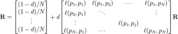
So, the equation is as follows:

$PR(p_i) = \frac{1-d}{N} + d \sum_{p_j \in M(p_i)} \frac{PR (p_j)}{L(p_j)}$

where $p_1, p_2, ..., p_N$ are the pages under consideration, $M(p_i)$ is the set of pages that link to $p_i$ , $L(p_j)$ is the number of outbound links on page $p_j$ , and N is the total number of pages.
The PageRank values are the entries of the dominant eigenvector of the modified adjacency matrix. This makes PageRank a particularly elegant metric: the eigenvector is

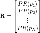
$\mathbf{R} = \begin{bmatrix} PR(p_1) \\ PR(p_2) \\ \vdots \\ PR(p_N) \end{bmatrix}$

where R is the solution of the equation

$\mathbf{R} = \begin{bmatrix} {(1-d)/ N} \\ {(1-d) / N} \\ \vdots \\ {(1-d) / N} \end{bmatrix} + d \begin{bmatrix} \ell(p_1,p_1) & \ell(p_1,p_2) & \cdots & \ell(p_1,p_N) \\ \ell(p_2,p_1) & \ddots & & \vdots \\ \vdots & & \ell(p_i,p_j) & \\ \ell(p_N,p_1) & \cdots & & \ell(p_N,p_N) \end{bmatrix} \mathbf{R}$

where the adjacency function $\ell(p_i,p_j)$ is 0 if page $p_j$ does not link to $p_i$ , and normalized such that, for each j

$\sum_{i = 1}^N \ell(p_i,p_j) = 1$ ,

i.e. the elements of each column sum up to 1, so the matrix is a stochastic matrix (for more details see the computation section below). Thus this is a variant of the eigenvector centrality measure used commonly in network analysis.
Because of the large eigengap of the modified adjacency matrix above the values of the PageRank eigenvector can be approximated to within a high degree of accuracy within only a few iterations.
As a result of Markov theory, it can be shown that the PageRank of a page is the probability of arriving at that page after a large number of clicks. This happens to equal $t^{-1}$ where $t$ is the expectation of the number of clicks (or random jumps) required to get from the page back to itself.
One main disadvantage of PageRank is that it favors older pages. A new page, even a very good one, will not have many links unless it is part of an existing site (a site being a densely connected set of pages, such as Wikipedia).
Several strategies have been proposed to accelerate the computation of PageRank.
Various strategies to manipulate PageRank have been employed in concerted efforts to improve search results rankings and monetize advertising links. These strategies have severely impacted the reliability of the PageRank concept, which purports to determine which documents are actually highly valued by the Web community.
Since December 2007, when it started actively penalizing sites selling paid text links, Google has combatted link farms and other schemes designed to artificially inflate PageRank. How Google identifies link farms and other PageRank manipulation tools is among Google's trade secrets.

Computation

PageRank can be computed either iteratively or algebraically. The iterative method can be viewed as the power iteration method or the power method. The basic mathematical operations performed are identical.

Iterative

At $t=0$ , an initial probability distribution is assumed, usually

$PR(p_i; 0) = \frac{1}{N}$ .

At each time step, the computation, as detailed above, yields

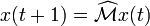
$PR(p_i;t+1) = \frac{1-d}{N} + d \sum_{p_j \in M(p_i)} \frac{PR (p_j; t)}{L(p_j)}$ ,

or in matrix notation

$\mathbf{R}(t+1) = d \mathcal{M}\mathbf{R}(t) + \frac{1-d}{N} \mathbf{1}$ , (*)

where $\mathbf{R}_i(t)=PR(p_i; t)$ and $\mathbf{1}$ is the column vector of length $N$ containing only ones.
The matrix $\mathcal{M}$ is defined as

$\mathcal{M}_{ij} = \begin{cases} 1 /L(p_j) , & \mbox{if }j\mbox{ links to }i\ \\ 0, & \mbox{otherwise} \end{cases}$

i.e.,

$\mathcal{M} := (K^{-1} A)^T$ ,

where $A$ denotes the adjacency matrix of the graph and $K$ is the diagonal matrix with the outdegrees in the diagonal.
The computation ends when for some small $\epsilon$

$|\mathbf{R}(t+1) - \mathbf{R}(t)| < \epsilon$ ,

i.e., when convergence is assumed.

Algebraic

For $t \to \infty$ (i.e., in the steady state), the above equation (*) reads

$\mathbf{R} = d \mathcal{M}\mathbf{R} + \frac{1-d}{N} \mathbf{1}$ . (**)

The solution is given by

$\mathbf{R} = (\mathbf{I}-d \mathcal{M})^{-1} \frac{1-d}{N} \mathbf{1}$ ,

with the identity matrix $\mathbf{I}$ .
The solution exists and is unique for $0 < d < 1$ . This can be seen by noting that $\mathcal{M}$ is by construction a stochastic matrix and hence has an eigenvalue equal to one as a consequence of the Perron–Frobenius theorem.

Power Method

If the matrix $\mathcal{M}$ is a transition probability, i.e., column-stochastic with no columns consisting of just zeros and $\mathbf{R}$ is a probability distribution (i.e., $|\mathbf{R}|=1$ , $\mathbf{E}\mathbf{R}=1$ where $\mathbf{E}$ is matrix of all ones), Eq. (**) is equivalent to

$\mathbf{R} = \left( d \mathcal{M} + \frac{1-d}{N} \mathbf{E} \right)\mathbf{R} =: \widehat{ \mathcal{M}} \mathbf{R}$ . (***)

Hence PageRank $\mathbf{R}$ is the principal eigenvector of $\widehat{\mathcal{M}}$ . A fast and easy way to compute this is using the power method: starting with an arbitrary vector $x(0)$ , the operator $\widehat{\mathcal{M}}$ is applied in succession, i.e.,

$x(t+1) = \widehat{\mathcal{M}} x(t)$ ,

until

$|x(t+1) - x(t)| < \epsilon$ .

Note that in Eq. (***) the matrix on the right-hand side in the parenthesis can be interpreted as

$\frac{1-d}{N} \mathbf{I} = (1-d)\mathbf{P} \mathbf{1}^t$ ,

where $\mathbf{P}$ is an initial probability distribution. In the current case

$\mathbf{P} := \frac{1}{N} \mathbf{1}$ .

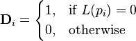
Finally, if $\mathcal{M}$ has columns with only zero values, they should be replaced with the initial probability vector $\mathbf{P}$ . In other words

$\mathcal{M}^\prime := \mathcal{M} + \mathcal{D}$ ,

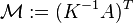
where the matrix $\mathcal{D}$ is defined as

$\mathcal{D} := \mathbf{P} \mathbf{D}^t$ ,

with

$\mathbf{D}_i = \begin{cases} 1, & \mbox{if }L(p_i)=0\ \\ 0, & \mbox{otherwise} \end{cases}$

In this case, the above two computations using $\mathcal{M}$ only give the same PageRank if their results are normalized:

$\mathbf{R}_{\textrm{power}} = \frac{\mathbf{R}_{\textrm{iterative}}}{|\mathbf{R}_{\textrm{iterative}}|} = \frac{\mathbf{R}_{\textrm{algebraic}}}{|\mathbf{R}_{\textrm{algebraic}}|}$ .

PageRank of an undirected graph

The PageRank of an undirected graph G is statistically close to the degree distribution of the graph G but they are generally not identical: If R is the PageRank vector defined above, and D is the degree distribution vector

$D = {1\over 2|E|} \begin{bmatrix} deg(p_1) \\ deg(p_2) \\ \vdots \\ deg(p_N) \end{bmatrix}$

where $deg(p_i)$ denotes the degree of vertex $p_i$ , and E is the edge-set of the graph, then, with $Y={1\over N}\mathbf{1}$ , by:

${1-d\over1+d}\|Y-D\|_1\leq \|R-D\|_1\leq \|Y-D\|_1,$

E-ask-how

I know you all are interested to learn something new i thing you are in the right Place.

Pages

Monday, 20 May 2013

At sky Guitar Chords

Monday, 22 April 2013

Love wallpaper

Awesome Facebook Cover photo

History of Facebook

How to count PageRank

Algorithm

Simplified algorithm

Damping factor

Computation

Iterative

Algebraic

Power Method

PageRank of an undirected graph

Popular Posts

Blogger templates

Blog Archive

Categories

Followers